Jordan Neural Network

Introduction

Like Elman Neural Networks, Jordan Neural Networks are also a simple recurrent neural network. They have proven to be a popular tool for applied time series modeling and are often trained alongside Elman because the two are very similar.

Jordan Neural Networks have a single hidden layer. The only difference between Elman and Jordan is that the context layer neurons are fed from the output layer instead of the hidden layer. Thus, Jordan “remembers” the output from the previous time-step.

Like Elman, Jordan neural networks are useful for predicting time series observations which have a short-term memory.

Data Preparation

First, we take log and then scale the data to a range of [0,1]. Then, we use quantmod package to create 12 time lagged attributes (12 because the data is monthly).

data = read.csv("data.csv")[,3]
data = ts(data, start = c(2001, 1), frequency = 12)
#
date = read.csv("data.csv")[,1]
date = as.Date(date, format = "%d/%m/%Y")

#Log-Transformation
y = ts(log(data), start = c(2001, 1), frequency = 12)

#Normalization
range.data = function(x){(x-min(x))/(max(x)-min(x))}
min.data = min(y) #12.57856
max.data = max(y) #14.10671
y = range.data(y)
unscale.data = function(x, xmin, xmax){x*(xmax-xmin)+xmin}

#Lag Selection
require(quantmod)
y  = as.zoo(y)
x1  = Lag(y, k = 1)
x2  = Lag(y, k = 2)
x3  = Lag(y, k = 3)
x4  = Lag(y, k = 4)
x5  = Lag(y, k = 5)
x6  = Lag(y, k = 6)
x7  = Lag(y, k = 7)
x8  = Lag(y, k = 8)
x9  = Lag(y, k = 9)
x10 = Lag(y,k = 10)
x11 = Lag(y,k = 11)
x12 = Lag(y,k = 12)
x  = cbind(x1,x2,x3,x4,x5,x6,x7,x8,x9,x10,x11,x12)
x  = cbind(y, x)
x  = x[-(1:12),] #Missing Value Removal
n  = nrow(x)     #236 observations
#
n.train = 224
train = 1:(n-12)
outputs = x$y
inputs = x[, 2:13]
#
require(RSNNS)

Training Model

To train the network, we use 224 values. The first 12 values were removed so that we have values at all the lags we use.

The package RSNNS contains function jordan which estimates an Jordan Neural Network.

The 1st argument takes in the lagged attributes contained in inputs object. “[train]” is used to specify training values.
The 2nd argument takes in the the values of observed time series.
The argument size specifies the number of nodes in each hidden layer
The argument maxit controls the number of iterations over which the network is optimized.
The argument learnFuncParams sets the learning rate. We use a low learning rate of 0.01 for all models.

We build 3 models with different number of nodes in the hidden layers.

The 1st model has 64 nodes optimized over 1000 iterations.
The 2nd model has 106 nodes optimized over 1000 iterations.
The 3rd model has 109 nodes optimized over 1000 iterations.

#
set.seed(2018)
fit1 = jordan(inputs[train], outputs[train], size = 64, learnFuncParams = c(0.01),maxit = 1000)
#
set.seed(2018)
fit2 = jordan(inputs[train], outputs[train], size = 106, learnFuncParams = c(0.01),maxit = 1000)
#
set.seed(2018)
fit3 = jordan(inputs[train], outputs[train], size = 109, learnFuncParams = c(0.01),maxit = 1000)

Iterative Error and Correlation Plot

The plotIterativeError function plots the iterative error over the sample.
The plotRegressionError function helps visualize the relationship between the Actual and Predicted values.

Note: Only the code for first plot is shown, other 2 plots are created with the same code.

par(mfrow=c(1,2))
plotIterativeError(fit1)
plotRegressionError(outputs[1:n.train,], fit1$fitted.values)
par(mfrow=c(1,1))
title("Model 1 Error and Fit")

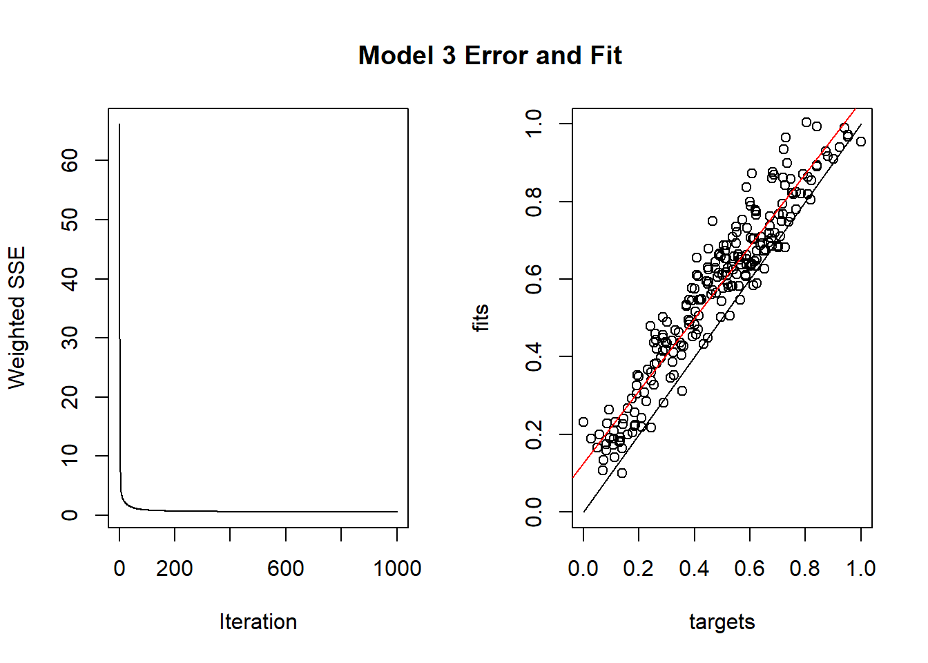
For the plot on the left, A rapidly decreasing error indicates that the model is learning from the available data.
For all the 3 models, the errors fall rapidly and then stays the same more or less.
For the plot on the right, we have a red and a black line. The solid black line indicates a perfect fit while the red line shows the actual linear fit to actual data.
The closer the red and black lines are, the better is the model.

Prediction

We use the predict function to make predictions. Now, because we had taken log and normalized all values, the predicted ones are not in original units.

To convert them back to original units, we take exponential and unscale them using a user-define function. We do the same with the actual test data values as well.

# Prediction
pred1 = predict(fit1, inputs[-train])
output.pred1 = exp(unscale.data(pred1, min.data, max.data))

pred2 = predict(fit2, inputs[-train])
output.pred2 = exp(unscale.data(pred2, min.data, max.data))

pred3 = predict(fit3, inputs[-train])
output.pred3 = exp(unscale.data(pred3, min.data, max.data))

# Actual Data
output.actual = exp(unscale.data(outputs[225:236], min.data, max.data))
output.actual = as.matrix(output.actual)
pred.dates = rownames(output.actual) #Prediction Dates
#
result = cbind(as.ts(output.actual), # Actual 
               as.ts(output.pred1),  # Model.1
               as.ts(output.pred2),  # Model.2
               as.ts(output.pred3))  # Model.3

RMSE-MAPE

library(Metrics)
round(c( mape(result$Actual, result$Model.1), 
         rmse(result$Actual, result$Model.1),
         
         mape(result$Actual, result$Model.2), 
         rmse(result$Actual, result$Model.2),
         
         mape(result$Actual, result$Model.3), 
         rmse(result$Actual, result$Model.3) ),5)

## [1]     0.07592 74657.97582     0.09367 93776.58728     0.05725 71608.57912

Ideally we want RMSE-MAPE figures to be as low as possible.
As per RMSE and MAPE, Model 3 (109 nodes) is a good fit.

Plot of All 3 Networks

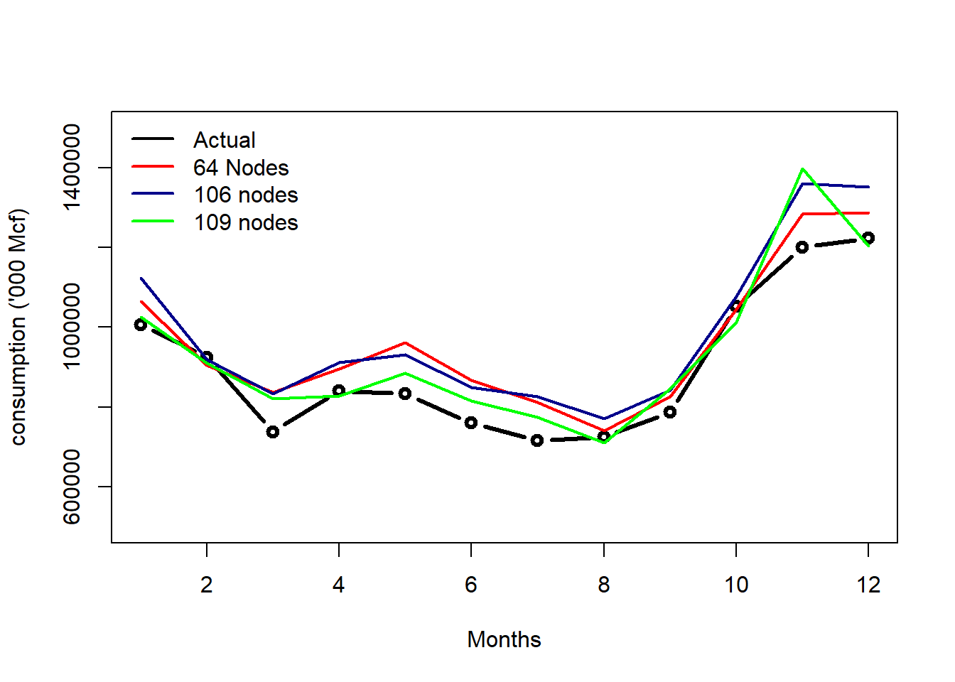
Overall, the Jordan Neural Network is able to capture the trend, seasonality and most of the underlying dynamics of our time series data.

Output Table

U.S. Consumption of Electricity Generated by Natural Gas
Dates	Actual¹	Model 1¹	Model 2¹	Model 3¹
Sep 2020	1006071.1	1064280.4	1122930.6	1025189.8
Oct 2020	924056.2	904008.6	918533.6	909775.6
Nov 2020	737935.2	837158.3	832361.0	819863.2
Dec 2020	839912.6	895515.0	912376.2	828382.0
Jan 2021	833783.3	962217.8	930818.0	885501.5
Feb 2021	759358.2	866818.8	849875.3	815062.7
Mar 2021	715165.1	811165.7	826456.9	773812.0
Apr 2021	724125.8	740006.6	771464.3	710971.7
May 2021	787027.2	826697.5	841688.4	845217.3
Jun 2021	1051774.8	1044398.2	1077180.5	1012727.0
Jul 2021	1199673.3	1283053.1	1359408.4	1398298.0
Aug 2021	1223328.0	1287099.5	1350961.4	1204196.9
Source: US Energy Information Adminstration
¹ Thousand Mcf