Recurrent Neural Network

Introduction

Recurrent Neural Networks come into picture when any model needs context to be able to provide an output based on the input. When we are dealing with Time series data, we know the future values are affected by the past values.

The RNN networks have a “memory”, it is able to remember what it has calculated so far. In order to achieve this, the RNN network has a loop which allows information to persist over time. While we input \(X_t\) and an output \(Y_t\) is generated at time ‘t’, the RNN also generates an internal state update \(h_t\) which contains information the internal state. This information is passed on to the next time step ‘t + 1’. Such networks with loops in them are called Recurrent because information is passed from one time step ‘t’ to another ‘t + 1’, internally within the network.

How does this happen?

If we look at the unrolled version above. First, it takes x(0) from the data and then outputs y(0) while generating h(0). In the next time step, h(0) and x(1) are input to generate x(2). This way, it keeps remembering context while training.

The RNN, by using a simple recurrence relation \(h_t = f_w(h_{t-1}, x_t)\) is able to process sequential data. At each time step t, the RNN generates the internal state \(h_t\) which is a function of the previous internal state and current input. It then applies a function ‘f’ which is parameterised by weights w. This function ‘f’ is the activation function say sigmoid or tanh or ReLu.

Back Propagation Through Time (BPTT)

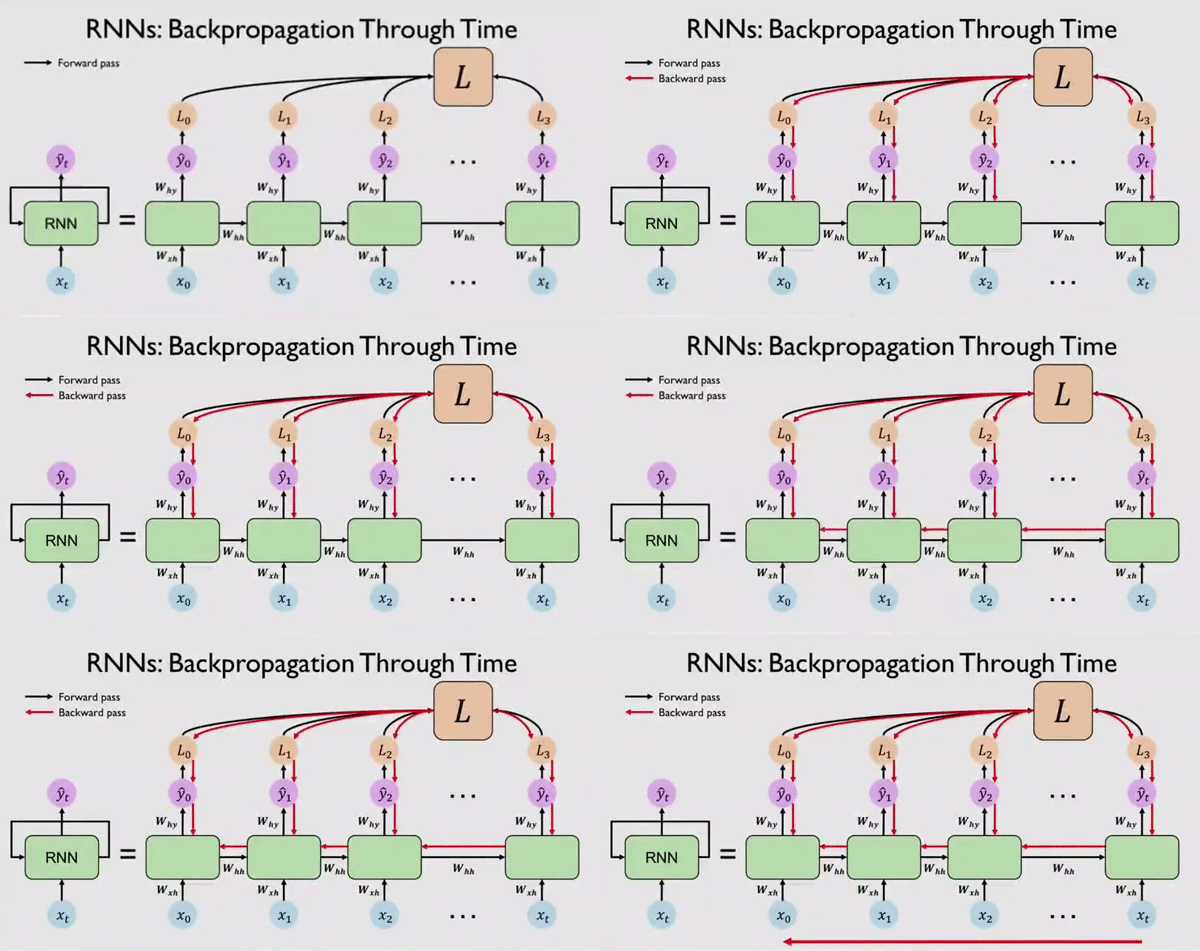
Along with output \(Y_t\) the network also generates an error/loss \(L_t\) at every time step. We can sum these individual losses to get a Total Loss \(L\). This Total Loss \(L\) should be minimized so that we have a good fit. For this, the RNN network, backpropagates errors at each individual time step and finally across all time steps all the way back from where we are currently to the beginning of the sequence. This process is called BPTT because all errors are flowing back in time to the beginning of our data sequence.

Data Preparation

We need to manipulate the data into a format which the Neural Network can work with. First, we use quantmod package to create 12 time lagged attributes (12 because the data is monthly).

After selecting necessary lags, we can take Log to sort of reduce the magnitude of the series and then Normalize the data to bring them in the range of 0 and 1.

  data = read.csv("data.csv")[,3]
  date = read.csv("data.csv")[,1]
  
  require(quantmod)
  x = as.zoo(data)
  
  # Selecting Lags
  x1   = Lag(x , k=1)
  x2   = Lag(x , k=2)
  x3   = Lag(x , k=3)
  x4   = Lag(x , k=4)
  x5   = Lag(x , k=5)
  x6   = Lag(x , k=6)
  x7   = Lag(x , k=7)
  x8   = Lag(x , k=8)
  x9   = Lag(x , k=9)
  x10  = Lag(x ,k=10)
  x11  = Lag(x ,k=11)
  x12  = Lag(x ,k=12)
  x    = cbind(x1,x2,x3,x4,x5,x6,x7,x8,x9,x10,x11,x12,x)
  
  # Log-transformation
  x  = log(x) 
  
  # Missing Value Removal
  x  = x [-(1:12),]
  x  = data.matrix(x)
  
  # Normalization
  min.xng = min(x) #12.57856
  max.xng = max(x) #14.10671
  x  = (x - min(x))/(max(x) - min(x))
  unscale = function(x,xmax, xmin){ x*(xmax-xmin)+ xmin }
  #
  x1  = as.matrix(x [,1])
  x2  = as.matrix(x [,2])
  x3  = as.matrix(x [,3])
  x4  = as.matrix(x [,4])
  x5  = as.matrix(x [,5])
  x6  = as.matrix(x [,6])
  x7  = as.matrix(x [,7])
  x8  = as.matrix(x [,8])
  x9  = as.matrix(x [,9])
  x10 = as.matrix(x[,10])
  x11 = as.matrix(x[,11])
  x12 = as.matrix(x[,12])
  y   = as.matrix(x[,13])
  #
  n.train = 224
  
  #Preparing Train dataset
  ytrain    = as.matrix(y [1:n.train])
  x1_train  = as.matrix(t(x1 [1:n.train,]))
  x2_train  = as.matrix(t(x2 [1:n.train,]))
  x3_train  = as.matrix(t(x3 [1:n.train,]))
  x4_train  = as.matrix(t(x4 [1:n.train,]))
  x5_train  = as.matrix(t(x5 [1:n.train,]))
  x6_train  = as.matrix(t(x6 [1:n.train,]))
  x7_train  = as.matrix(t(x7 [1:n.train,]))
  x8_train  = as.matrix(t(x8 [1:n.train,]))
  x9_train  = as.matrix(t(x9 [1:n.train,]))   
  x10_train = as.matrix(t(x10[1:n.train,]))
  x11_train = as.matrix(t(x11[1:n.train,]))
  x12_train = as.matrix(t(x12[1:n.train,]))
  #
  x_train  = array(c(x1_train,x2_train,x3_train,x4_train,x5_train,x6_train,
                    x7_train,x8_train,x9_train,x10_train,x11_train,x12_train)
                   ,dim = c(dim(x1_train),12))
  
  #Preparing Test dataset
  x1test  = as.matrix(t(x1 [(n.train+1):nrow(x1), ]))
  x2test  = as.matrix(t(x2 [(n.train+1):nrow(x2), ]))
  x3test  = as.matrix(t(x3 [(n.train+1):nrow(x3), ]))
  x4test  = as.matrix(t(x4 [(n.train+1):nrow(x4), ]))
  x5test  = as.matrix(t(x5 [(n.train+1):nrow(x5), ]))
  x6test  = as.matrix(t(x6 [(n.train+1):nrow(x6), ]))
  x7test  = as.matrix(t(x7 [(n.train+1):nrow(x7), ]))
  x8test  = as.matrix(t(x8 [(n.train+1):nrow(x8), ]))
  x9test  = as.matrix(t(x9 [(n.train+1):nrow(x9), ]))
  x10test = as.matrix(t(x10[(n.train+1):nrow(x10),]))
  x11test = as.matrix(t(x11[(n.train+1):nrow(x11),]))
  x12test = as.matrix(t(x12[(n.train+1):nrow(x12),]))
  ytest   = as.matrix(y [(n.train+1):nrow(x12 )])
  xtest   = array(c(x1test,x2test,x3test,x4test,x5test,x6test,
                    x7test,x8test,x9test,x10test,x11test,x12test),
                  dim = c(dim(x1test), 12))

require(rnn)

RNN Model

The model is estimated using the trainr function in the RNN package. It requires the attribute data be passed as a 3 dimensional array. The first dimension is the number of samples, the second dimension time, and the third dimension captures the variables. This is reflected by xtest object.

We use set.seed(2018) through out to allow reproducibility.

The RNN network is specified by network_type = “rnn”.

We will build 3 models with different values of hidden_dim which tells how many layers and neurons are there in the network. All models have the same learning rate of 0.05 and sigmoid activation function.

1st model consists of 15 nodes in the hidden layer. The network is optimized over 500 epochs.
2nd model consists of (9 and 3) nodes in the first and second hidden layers respectively, but optimized over 300 epochs.
3rd model consists of (5 and 2) nodes in the first and second hidden layers respectively, but optimized over 550 epochs.

#
set.seed(2018)
model1  = trainr(Y = t(ytrain), X = x_train , learningrate = 0.05,
                 hidden_dim = 15, numepochs = 500,
                 network_type = "rnn",sigmoid = "logistic")
#
set.seed(2018)
model2  = trainr(Y = t(ytrain), X = x_train , learningrate = 0.05,
                 hidden_dim = c(9,3) , numepochs = 300,
                 network_type = "rnn",sigmoid = "logistic")
#
set.seed(2018)
model3  = trainr(Y = t(ytrain), X = x_train , learningrate = 0.05, 
                 hidden_dim = c(5,2) , numepochs = 550,
                 network_type = "rnn",sigmoid = "logistic")

Plot of Iterative Error

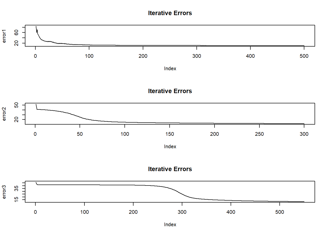
As the model is training, it output an error figure. Here we plot these errors and iteration index.

error1  = t(model1 $error)
error2  = t(model2$error)
error3  = t(model3$error)
#
par(mfrow=c(3,1))
plot(error1, type="l", main="Iterative Errors")
plot(error2, type="l", main="Iterative Errors")
plot(error3, type="l",main="Iterative Errors")

If the plots show a fall in error with increasing iteration, it means that the network is learning.
If the plots show a sudden spike at say 200th iteration, we should stop and change the numepochs to 200 because beyond 200, the network is overfitting on the training data.
Here, all three plots are more or less satisfactory.

Prediction

We use the _predictr_ function to make predictions.Now because we had taken log and normalized, the predicted values are not in original but log-scaled units.

To convert them back to original units, we take exponential and unscale them using a user-define function. We do the same with the actual test data values as well.

# Prediction
pred1test  = t(predictr(model1, xtest))
pred1.act  = exp(unscale(pred1test, max.xng, min.xng))
pred1.act  = ts(matrix(pred1.act), end = c(2020,8), frequency = 12)

pred2test  = t(predictr(model2, xtest))
pred2.act  = exp(unscale(pred2test, max.xng, min.xng))
pred2.act  = ts(matrix(pred2.act), end = c(2020,8), frequency = 12)

pred3test  = t(predictr(model3, xtest))
pred3.act  = exp(unscale(pred3test,max.xng, min.xng))
pred3.act  = ts(matrix(pred3.act), end = c(2020,8), frequency = 12)

# Actual Data
y.act  = exp(unscale(ytest , max.xng, min.xng))
y.act  = ts(matrix(y.act), end = c(2020,8), frequency = 12)

# Final Output  
result = cbind(date[237:248],     # Prediction Dates
               round(y.act,2),    # Test data
               round(pred1.act,2),# Model.1
               round(pred2.act,2),# Model.2
               round(pred3.act,2))# Model.3

Plot of All 3 Networks

We can say that all three models have more or less captured the underlying dynamics of the data.

RMSE-MAPE

library(Metrics)
round(c( mape(result$actual, result$model1), 
         rmse(result$actual, result$model1), 

         mape(result$actual, result$model2), 
         rmse(result$actual, result$model2), 

         mape(result$actual, result$model3),
         rmse(result$actual, result$model3) ), 5)

## [1]     0.08477 88893.05230     0.07977 96615.96953     0.08900 99173.33448

As per RMSE, Model 2 (with 9,3 nodes in 2 hidden layers) is a good fit.
As per MAPE, Model 1 (with 42 nodes in a single hidden layer) is a good fit.
Ideally we want RMSE-MAPE figures to be as low as possible.

Output Table

U.S. Consumption of Electricity Generated by Natural Gas
Date	Actual¹	model_1¹	model_2¹	model_3¹
Sep 1, 2020	1006071.2	1104944.6	943044.0	1077797.8
Oct 1, 2020	924056.2	929203.7	925937.0	947461.9
Nov 1, 2020	737935.2	882783.3	869885.1	885618.1
Dec 1, 2020	839912.6	865456.6	872521.1	838168.7
Jan 1, 2021	833783.3	891370.7	871471.2	883557.2
Feb 1, 2021	759358.2	873895.0	850812.1	841373.4
Mar 1, 2021	715165.1	803378.6	767081.0	767787.8
Apr 1, 2021	724125.8	729239.0	722215.3	759326.4
May 1, 2021	787027.2	844170.5	816924.2	868377.9
Jun 1, 2021	1051774.8	996437.3	949022.0	963258.8
Jul 1, 2021	1199673.3	1077251.3	1029848.8	1035439.0
Aug 1, 2021	1223328.0	1089798.1	1031520.2	1033907.2
Source: US Energy Information Adminstration
¹ Thousand Mcf