Long Short-Term Memory
Introduction
Conventional RNNs suffer from short-term memory loss. Over time, input from earlier time steps become less significant. Hence, RNNs can fail to retain the context from those earlier steps of the data. The Back Propagation Through Time (BPTT) is the cause behind this short-term memory loss. Over time gradients becomes too small to the point they become insignificant for updating weights. The gradients keep shrinking in size and eventually “vanish”. This is called the Vanishing Gradient Problem. This makes it harder to propagate errors back into the past because the gradients are becoming smaller and smaller. Thus, we bias out network to capture more of short-term dependencies.
Long Short-Term Memory LSTMs are used to mitigate the issue of short-term memory through the use of gates that can regulate the flow of information passing through it.
Structure of Gate Cells
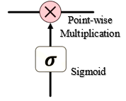
The Gate Cells consists of a neural net layer like a sigmoid and a point-wise multiplication. The Sigmoid translates it’s input over the range of [0, 1]. This translation can be thought of as How much of the passing information should be retained? where 0 means nothing and 1 means everything. Thus, in some sense, we are gating the flow of information.
Working of LSTMs
The working of LSTMs can be understood in 4 simple steps (1)Forget (2)Store (3)Update (4)Output.
- Forget
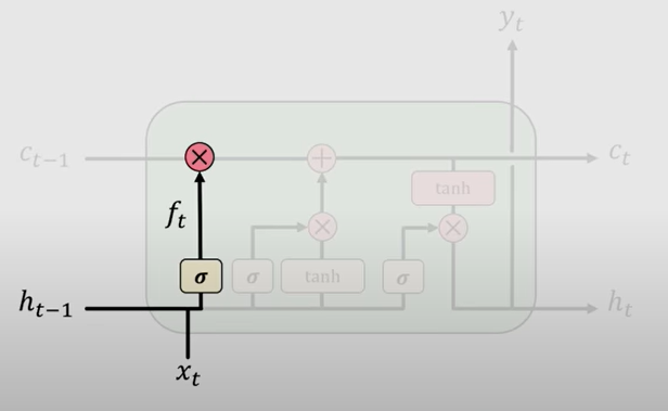
The first step in LSTMs is to decide what information is going to be thrown away/ from the cell state i.e. forgetting irrelevant history. This is a function of prior cell state \(h_{t-1}\) and current input \(x_t\).
- Store

The next step is to decide what part of the new information is relevant and then store it into the cell state.
- Update

Then it takes relevant parts of the prior and current information and uses this to selectively update the cell state.
- Output
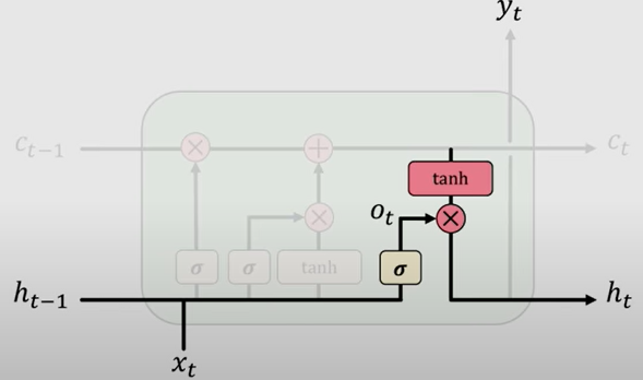
Finally it returns an output from what is known as the Output Gate which controls what information encoded in the cell state is sent to the network as input in the next time step.

Some resources for reference
Data Preparation
We need to manipulate the data into a format which the Neural Network can work with. First, we use quantmod package to create 12 time lagged attributes (12 because the data is monthly).
After selecting necessary lags, we can take Log to sort of reduce the magnitude of the series and then Normalize the data to bring them in the range of 0 and 1.
This part is the same as under RNN.
  data = read.csv("data.csv")[,3]
  date = read.csv("data.csv")[,1]

  require(quantmod)
  x = as.zoo(data)

  # Selecting Lags
  x1   = Lag(x , k=1)
  x2   = Lag(x , k=2)
  x3   = Lag(x , k=3)
  x4   = Lag(x , k=4)
  x5   = Lag(x , k=5)
  x6   = Lag(x , k=6)
  x7   = Lag(x , k=7)
  x8   = Lag(x , k=8)
  x9   = Lag(x , k=9)
  x10  = Lag(x ,k=10)
  x11  = Lag(x ,k=11)
  x12  = Lag(x ,k=12)
  x    = cbind(x1,x2,x3,x4,x5,x6,x7,x8,x9,x10,x11,x12,x)

  # Log-transformation
  x  = log(x)

  # Missing Value Removal
  x  = x [-(1:12),]
  x  = data.matrix(x)

  # Normalization
  min.xng = min(x) #12.57856
  max.xng = max(x) #14.10671
  x  = (x - min(x))/(max(x) - min(x))
  unscale = function(x,xmax, xmin){ x*(xmax-xmin)+ xmin }
  #
  x1  = as.matrix(x [,1])
  x2  = as.matrix(x [,2])
  x3  = as.matrix(x [,3])
  x4  = as.matrix(x [,4])
  x5  = as.matrix(x [,5])
  x6  = as.matrix(x [,6])
  x7  = as.matrix(x [,7])
  x8  = as.matrix(x [,8])
  x9  = as.matrix(x [,9])
  x10 = as.matrix(x[,10])
  x11 = as.matrix(x[,11])
  x12 = as.matrix(x[,12])
  y   = as.matrix(x[,13])
  #
  n.train = 224

  #Preparing Train dataset
  ytrain    = as.matrix(y [1:n.train])
  x1_train  = as.matrix(t(x1 [1:n.train,]))
  x2_train  = as.matrix(t(x2 [1:n.train,]))
  x3_train  = as.matrix(t(x3 [1:n.train,]))
  x4_train  = as.matrix(t(x4 [1:n.train,]))
  x5_train  = as.matrix(t(x5 [1:n.train,]))
  x6_train  = as.matrix(t(x6 [1:n.train,]))
  x7_train  = as.matrix(t(x7 [1:n.train,]))
  x8_train  = as.matrix(t(x8 [1:n.train,]))
  x9_train  = as.matrix(t(x9 [1:n.train,]))
  x10_train = as.matrix(t(x10[1:n.train,]))
  x11_train = as.matrix(t(x11[1:n.train,]))
  x12_train = as.matrix(t(x12[1:n.train,]))
  #
  x_train  = array(c(x1_train,x2_train,x3_train,x4_train,x5_train,
                  x6_train,x7_train,x8_train,x9_train,x10_train,
                  x11_train,x12_train),dim = c(dim(x1_train),12))

  #Preparing Test dataset
  x1test  = as.matrix(t(x1 [(n.train+1):nrow(x1), ]))
  x2test  = as.matrix(t(x2 [(n.train+1):nrow(x2), ]))
  x3test  = as.matrix(t(x3 [(n.train+1):nrow(x3), ]))
  x4test  = as.matrix(t(x4 [(n.train+1):nrow(x4), ]))
  x5test  = as.matrix(t(x5 [(n.train+1):nrow(x5), ]))
  x6test  = as.matrix(t(x6 [(n.train+1):nrow(x6), ]))
  x7test  = as.matrix(t(x7 [(n.train+1):nrow(x7), ]))
  x8test  = as.matrix(t(x8 [(n.train+1):nrow(x8), ]))
  x9test  = as.matrix(t(x9 [(n.train+1):nrow(x9), ]))
  x10test = as.matrix(t(x10[(n.train+1):nrow(x10),]))
  x11test = as.matrix(t(x11[(n.train+1):nrow(x11),]))
  x12test = as.matrix(t(x12[(n.train+1):nrow(x12),]))
  ytest   = as.matrix(y [(n.train+1):nrow(x12 )])
  xtest   = array(c(x1test,x2test,x3test,x4test,x5test,x6test,
                    x7test,x8test,x9test,x10test,x11test,x12test),
                  dim = c(dim(x1test), 12))

require(rnn)
LSTM Network
The model is estimated using the trainr function in the RNN package. It requires the attribute data be passed as a 3 dimensional array. The first dimension is the number of samples, the second dimension time, and the third dimension captures the variables. This is reflected by xtest object.
We use set.seed(2018) to allow reproducibility.
The LSTM network is specified by network_type = “lstm”.
We will build 3 models with different values of hidden_dim which tells how many layers and neurons are there in the network. All models have the same learning rate of 0.05 and sigmoid activation function.
- 1st model consists of 3 nodes in the hidden layer. The network is optimized over 500 epochs.
- 2nd model consists of 5 nodes in the hidden layer. The network is optimized over 300 epochs.
- 3rd model consists of 7 nodes in the hidden layer. The network is optimized over 300 epochs.
#
set.seed(2018)
model1  = trainr(Y = t(ytrain ), X = x_train , learningrate = 0.05,
                 hidden_dim = 3, numepochs = 500,
                 network_type = "lstm", sigmoid = "tanh")
#
set.seed(2018)
model2  = trainr(Y = t(ytrain), X = x_train , learningrate = 0.05,
                 hidden_dim = 5, numepochs = 300,
                 network_type = "lstm",sigmoid = "tanh")
#
set.seed(2018)
model3  = trainr(Y = t(ytrain ), X = x_train , learningrate = 0.05,
                 hidden_dim = 7, numepochs = 300,
                 network_type = "lstm", sigmoid = "tanh")
Plot of Iterative Error
As the model is training, it output an error figure. Here we plot these errors and iteration index.
error1  = t(model1 $error)
error2  = t(model2$error)
error3  = t(model3$error)
#
par(mfrow=c(3,1))
plot(error1, type="l", main="Iterative Errors")
plot(error2, type="l", main="Iterative Errors")
plot(error3, type="l",main="Iterative Errors")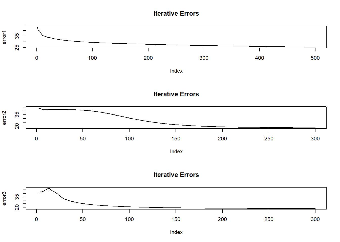
- If the plots show a fall in error with increasing iteration, it means that the network is learning.
- If the plots show a sudden spike at say 200th iteration, we should stop and change the numepochs to 200 because beyond 200, the network is overfitting on the training data.
- Here, all three plots are more or less satisfactory.
Prediction
We use the predictr function to predict and then unscale and take exponential to transform the predicted values back into original scale.
To convert them back to original units, we take exponential and unscale them using a user-define function. We do the same with the actual test data values as well.
# Prediction
pred1test = t(predictr(model1, xtest))
pred1.act  = exp(unscale(pred1test, max.xng, min.xng))
pred1.act  = ts(matrix(pred1.act), end = c(2020,8), frequency = 12)

pred2test = t(predictr(model2, xtest))
pred2.act  = exp(unscale(pred2test, max.xng, min.xng))
pred2.act  = ts(matrix(pred2.act), end = c(2020,8), frequency = 12)

pred3test = t(predictr(model3, xtest))
pred3.act  = exp(unscale(pred3test,max.xng, min.xng))
pred3.act  = ts(matrix(pred3.act), end = c(2020,8), frequency = 12)

# Actual Data
y.act  = exp(unscale(ytest , max.xng, min.xng))
y.act  = ts(matrix(y.act), end = c(2020,8), frequency = 12)

# Final Output
result = cbind(date[237:248],     # Prediction Dates
               round(y.act,2),    # Test data
               round(pred1.act,2),# Model.1
               round(pred2.act,2),# Model.2
               round(pred3.act,2))# Model.3
Plot of All 3 Networks
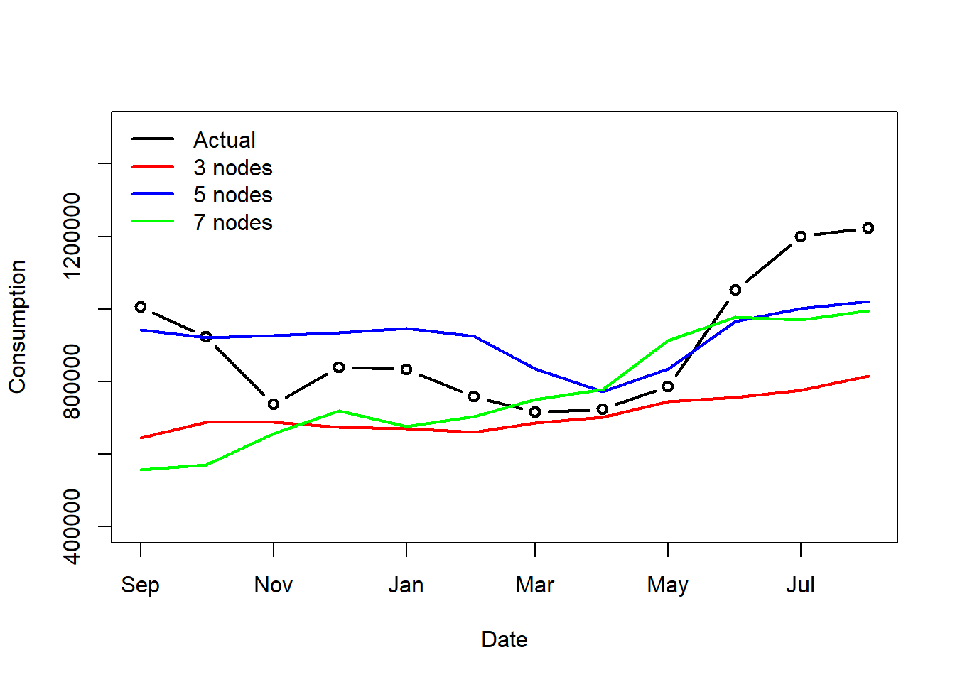
- The blue line (Model2) initially overestimates and then underestimates towards the end. The red and green line (Model 1 and 3) highly underestimate as well.
- There is a lot of under-prediction, looking at the values can make it even clearer.
- Clearly, this network performs poorly on our dataset.
RMSE-MAPE
library(Metrics)
round(c( mape(result$actual, result$model1),
         rmse(result$actual, result$model1),

         mape(result$actual, result$model2),
         rmse(result$actual, result$model2),

         mape(result$actual, result$model3),
         rmse(result$actual, result$model3) ), 3)
## [1] 0.192 239540.856 0.125 128035.842 0.173 205560.788- As per RMSE-MAPE, Model 2 (with 5 nodes in the hidden layer) is a best fit among the three.
- Ideally, we want RMSE-MAPE figures to be as low as possible.
- However, here all 3 models have quite high RMSE-MAPE values.
However, like many things in data science, there is no guarantee that this model will always deliver the best, or even acceptable performance on our data. The LSTM is only one of many emerging types of recurrent neural network useful for time series forecasting. - N.D. Lewis
Output Table
| U.S. Consumption of Electricity Generated by Natural Gas | ||||
|---|---|---|---|---|
| Date | Actual1 | model_11 | model_21 | model_31 |
| Sep 1, 2020 | 1006071.2 | 644952.7 | 942251.7 | 556579.6 |
| Oct 1, 2020 | 924056.2 | 687834.3 | 920977.7 | 570375.1 |
| Nov 1, 2020 | 737935.2 | 687563.0 | 927356.7 | 655922.9 |
| Dec 1, 2020 | 839912.6 | 674210.9 | 935679.9 | 719214.1 |
| Jan 1, 2021 | 833783.3 | 670159.3 | 947614.4 | 676637.1 |
| Feb 1, 2021 | 759358.2 | 660507.9 | 925421.6 | 704601.8 |
| Mar 1, 2021 | 715165.1 | 685644.8 | 835823.9 | 751415.4 |
| Apr 1, 2021 | 724125.8 | 701448.1 | 772442.4 | 777689.0 |
| May 1, 2021 | 787027.2 | 744133.4 | 834709.2 | 914212.4 |
| Jun 1, 2021 | 1051774.8 | 755805.3 | 966786.3 | 978336.4 |
| Jul 1, 2021 | 1199673.3 | 776137.9 | 1001214.5 | 969598.2 |
| Aug 1, 2021 | 1223328.0 | 816380.6 | 1020168.8 | 994733.2 |
| Source: US Energy Information Adminstration | ||||
|
1
Thousand Mcf
|
||||