Elman Neural Network
Introduction
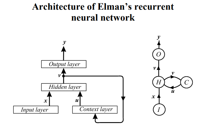
Elman Neural Network is a popular and simple recurrent neural network. It was designed to learn sequential or time-varying patterns. They consist of an Input layer, a context layer, a hidden layer and an output layer. Each layer contains one or more neurons which propagate information from one layer to another by computing a non-linear function of their weighted sum of inputs. The context layer’s presence leads to the Elman Neural Network having a “memory”.
In an Elman Neural Network, the number of neurons in the context layer is equal to the number of neurons in the hidden layer. In addition, the context layer neurons are fully connected to all neurons in the hidden layer.
Similar to a regular feedforward neural network, the strength of all connections between neurons is determined by a weight. Initially, all weights are chosen randomly and are optimized during training.
Data Preparation
First, we take log and then scale the data to a range of [0,1]. Then, we use quantmod package to create 12 time lagged attributes (12 because the data is monthly).
data = read.csv("data.csv")[,3]
data = ts(data, start = c(2001, 1), frequency = 12)
#
date = read.csv("data.csv")[,1]
date = as.Date(date, format = "%d/%m/%Y")

#Log-Transformation
y = ts(log(data), start = c(2001, 1), frequency = 12)

#Normalization
range.data = function(x){(x-min(x))/(max(x)-min(x))}
unscale.data = function(x, xmin, xmax){x*(xmax-xmin)+xmin}
min.data = min(y) #12.57856
max.data = max(y) #14.10671
y = range.data(y)

#Lag Selection
require(quantmod)
y   = as.zoo(y)
x1  = Lag(y, k = 1)
x2  = Lag(y, k = 2)
x3  = Lag(y, k = 3)
x4  = Lag(y, k = 4)
x5  = Lag(y, k = 5)
x6  = Lag(y, k = 6)
x7  = Lag(y, k = 7)
x8  = Lag(y, k = 8)
x9  = Lag(y, k = 9)
x10 = Lag(y,k = 10)
x11 = Lag(y,k = 11)
x12 = Lag(y,k = 12)
x   = cbind(x1,x2,x3,x4,x5,x6,x7,x8,x9,x10,x11,x12)
x   = cbind(y, x)
x   = x[-(1:12),] #Missing Value Removal
n   = nrow(x)     #236 observations
#
n.train = 224
outputs = x$y
inputs = x[ ,2:13]
#
require(RSNNS)
Training Model
To train the network, we use 224 values. The first 12 values were removed so that we have values at all the lags we use.
The package RSNNS contains function elman which estimates an Elman Neural Network.
- The 1st argument takes in the lagged attributes contained in inputs object. “1:n.train” is used to specify training values.
- The 2nd argument takes in the the values of observed time series.
- The argument size specifies the number of nodes in each hidden layer
- The argument maxit controls the number of iterations over which the network is optimized.
We build 3 models with different number of nodes in the hidden layers.
- The 1st model has 1 hidden layer with 42 nodes in a single hidden layer, optimized over 1000 iterations.
- The 2nd model has 2 hidden layers with 36 and 36 nodes, optimized over 1000 iterations.
- The 3rd model has 2 hidden layers with 15 and 14 nodes, optimized over 1000 iterations.
#
set.seed(2018)
fit1  = elman(inputs[1:n.train,], outputs[1:n.train,], size = 42, maxit = 1000)
#
set.seed(2018)
fit2  = elman(inputs[1:n.train,], outputs[1:n.train,], size = c(36,36), maxit = 1000)
#
set.seed(2018)
fit3  = elman(inputs[1:n.train,], outputs[1:n.train,], size = c(15,14), maxit = 1000)
#
Iterative Error and Correlation Plot
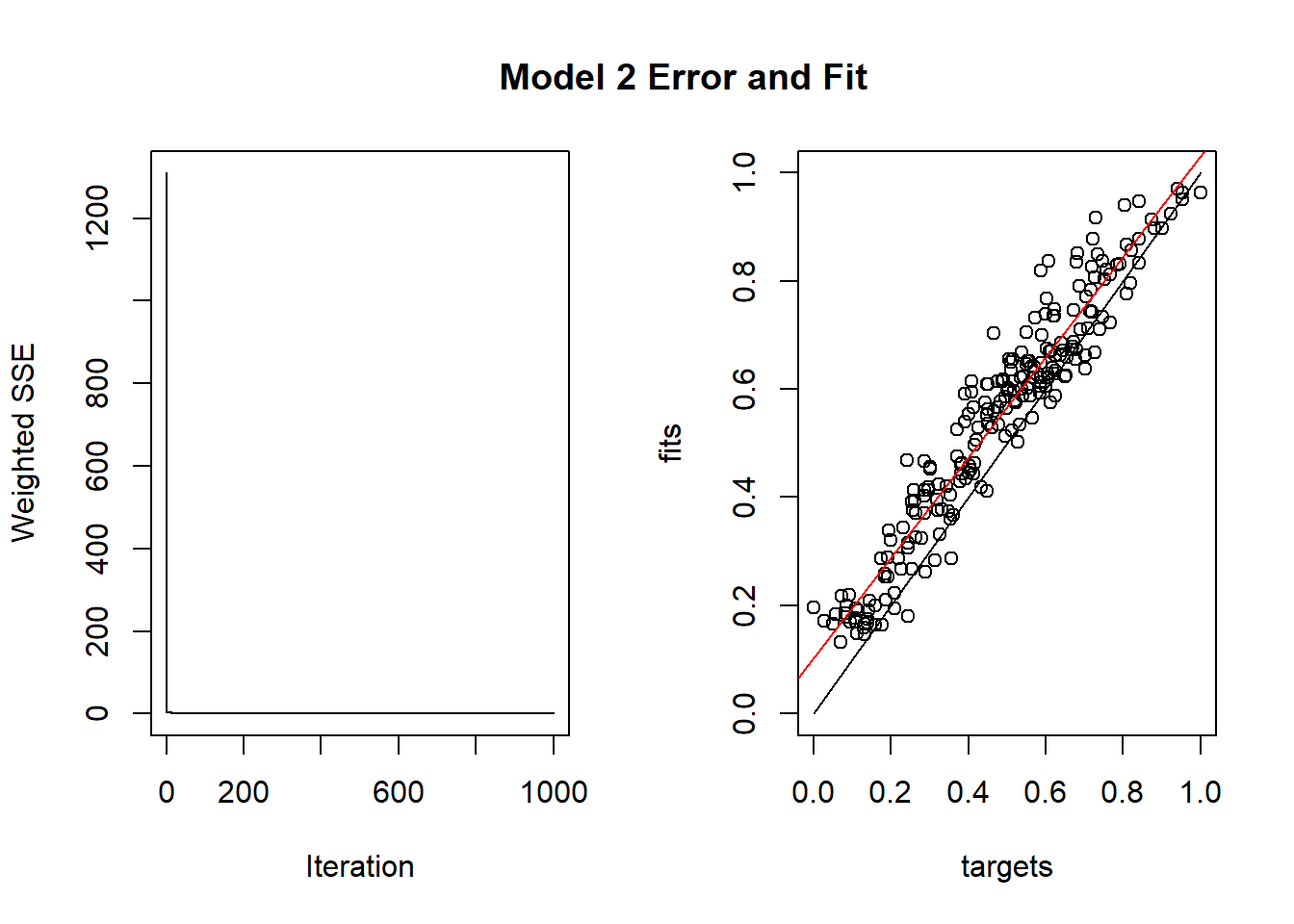
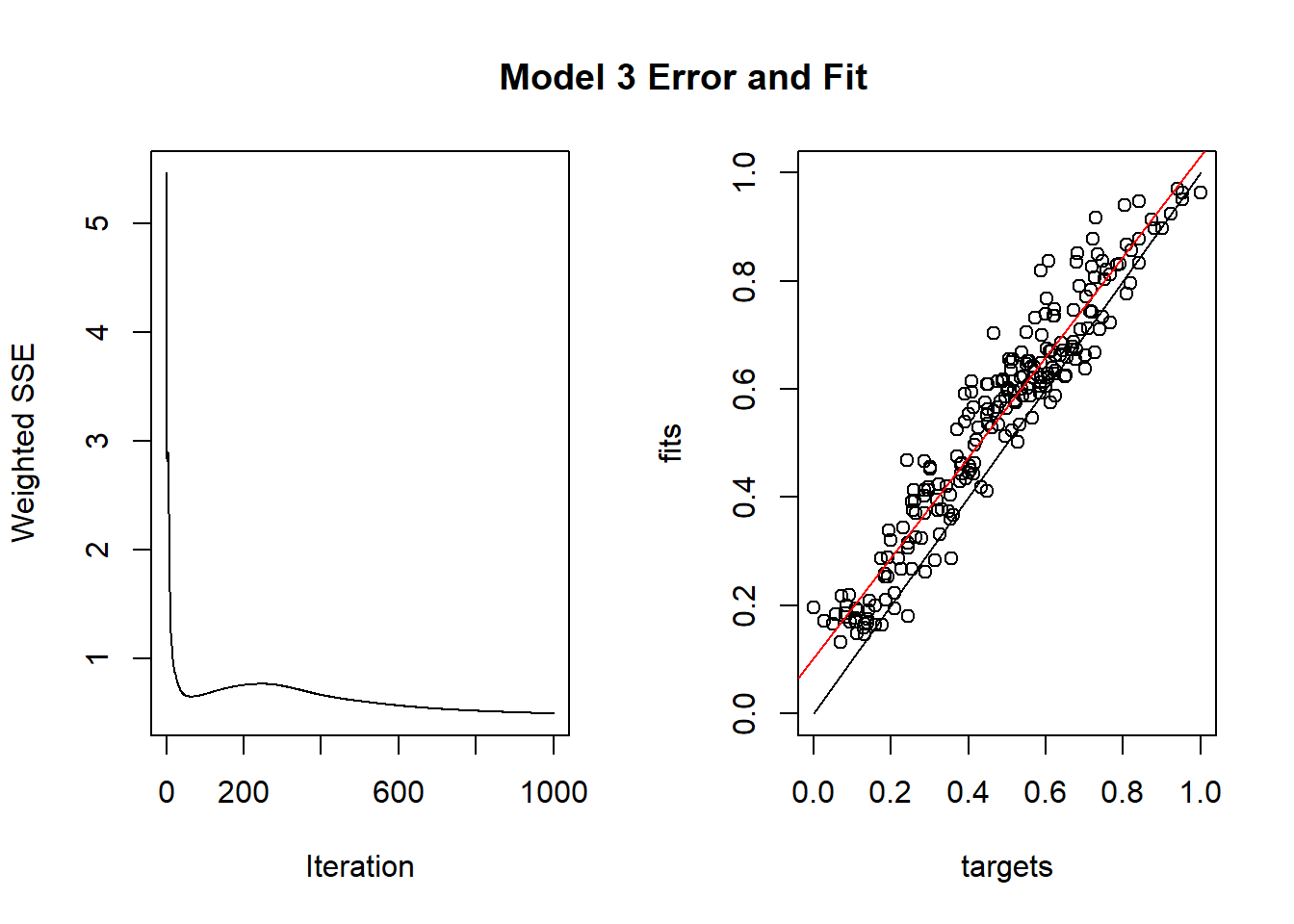
The plotIterativeError function plots the iterative error over the sample.
The plotRegressionError function helps visualize the relationship between the Actual and Predicted values.
Note: Only the code for first plot is shown, other 2 plots are created with the same code.
par(mfrow=c(1,2))
plotIterativeError(fit1)
plotRegressionError(outputs[1:n.train,], fit1$fitted.values)
par(mfrow=c(1,1))
title("Model 1 Error and Fit")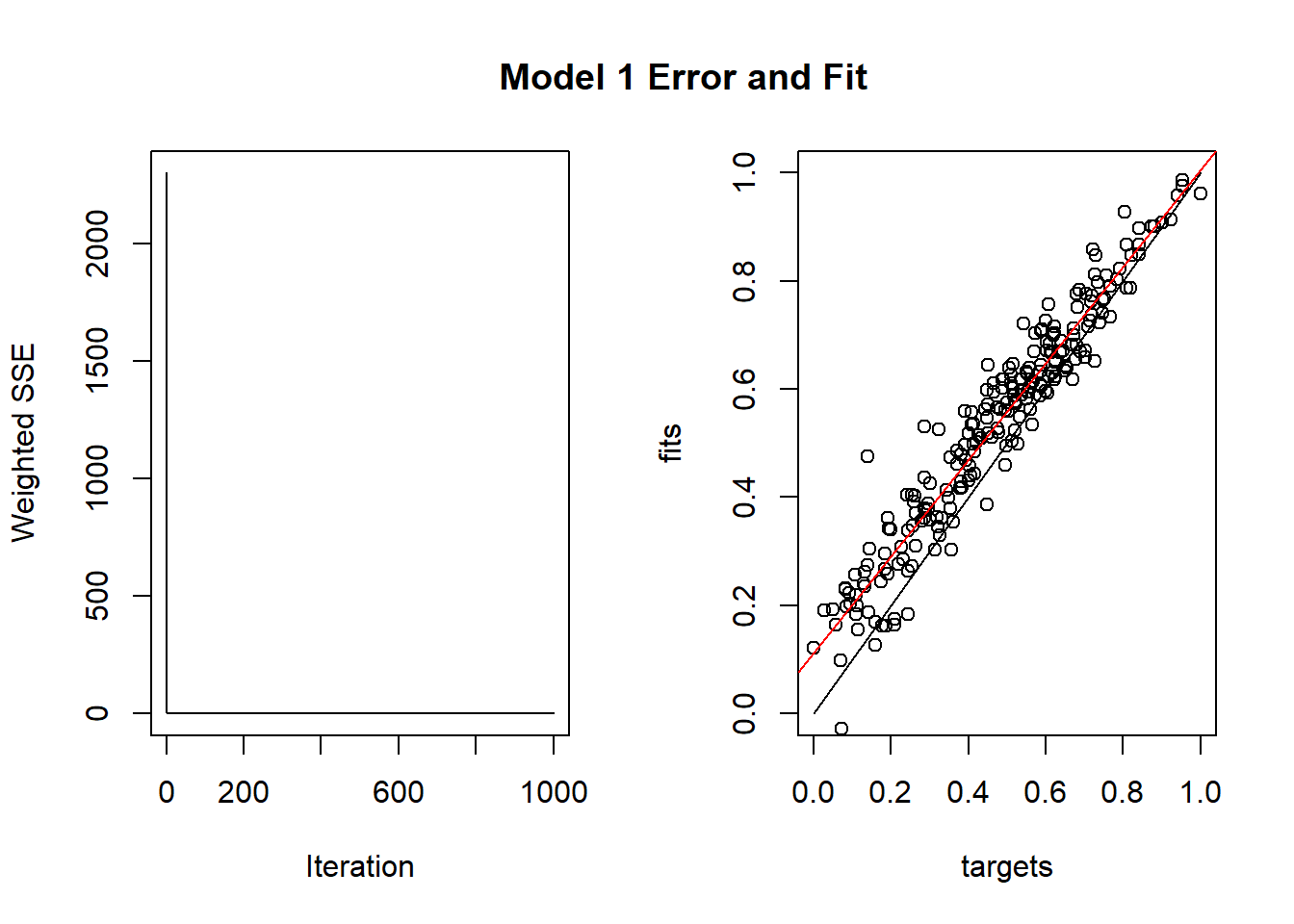
- For the plot on the left, A rapidly decreasing error indicates that the model is learning from the available data.
- For all the 3 models, the errors fall rapidly and then stays the same more or less.
- For the plot on the right, we have a red and a black line. The solid black line indicates a perfect fit while the red line shows the actual linear fit to actual data.
- The closer the red and black lines are, the better is the model.
Prediction
We use the predict function to make predictions. Now, because we had taken log and normalized all values, the predicted ones are not in original units.
To convert them back to original units, we take exponential and unscale them using a user-define function. We do the same with the actual test data values as well.
# Prediction
pred1 = predict(fit1, inputs[225:236])
output.pred1 = exp(unscale.data(pred1, min.data, max.data))

pred2 = predict(fit2, inputs[225:236])
output.pred2 = exp(unscale.data(pred2, min.data, max.data))

pred3 = predict(fit3, inputs[225:236])
output.pred3 = exp(unscale.data(pred3, min.data, max.data))

# Actual Data
output.actual = exp(unscale.data(outputs[225:236], min.data, max.data))
output.actual = as.matrix(output.actual)
pred.dates = rownames(output.actual) #Prediction Dates
#
result = cbind(as.ts(output.actual), # Actual
               as.ts(output.pred1),  # Model.1
               as.ts(output.pred2),  # Model.2
               as.ts(output.pred3))  # Model.3
RMSE-MAPE
library(Metrics)
round(c( mape(result$Actual, result$Model.1),
         rmse(result$Actual, result$Model.1),

         mape(result$Actual, result$Model.2),
         rmse(result$Actual, result$Model.2),

         mape(result$Actual, result$Model.3),
         rmse(result$Actual, result$Model.3) ),5)
## [1] 0.05251 54236.36921 0.05382 65440.61282 0.05241 55922.01240- As per RMSE, Model 3 (with 15 and 14 nodes) is a good fit.
- As per MAPE, Model 1 (with 42 nodes) is a good fit.
- Ideally we want RMSE-MAPE figures to be as low as possible.
Plot of All 3 Networks
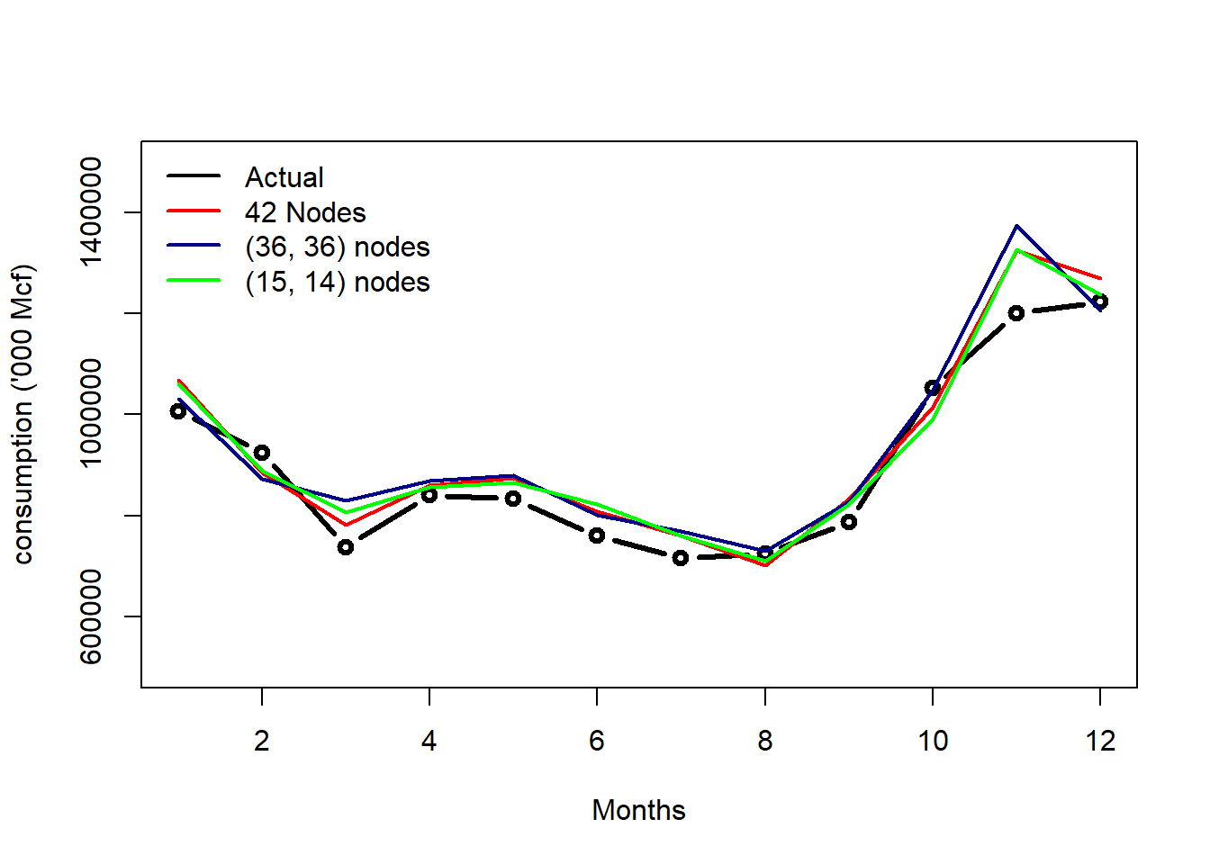
Overall, the Elman Neural Network is able to capture the trend, seasonality and most of the underlying dynamics our time series data.
Output Table
| U.S. Consumption of Electricity Generated by Natural Gas | ||||
|---|---|---|---|---|
| Dates | Actual1 | Model 11 | Model 21 | Model 31 |
| Sep 2020 | 1006071.1 | 1068077.4 | 1030405.7 | 1061165.1 |
| Oct 2020 | 924056.2 | 884531.1 | 872490.8 | 889184.2 |
| Nov 2020 | 737935.2 | 781011.9 | 829221.2 | 805831.3 |
| Dec 2020 | 839912.6 | 860308.1 | 868775.0 | 856287.5 |
| Jan 2021 | 833783.3 | 874707.5 | 879176.6 | 865947.3 |
| Feb 2021 | 759358.2 | 807957.9 | 801456.5 | 822646.1 |
| Mar 2021 | 715165.1 | 760154.4 | 768440.8 | 761077.9 |
| Apr 2021 | 724125.8 | 700721.5 | 729664.3 | 710964.2 |
| May 2021 | 787027.2 | 833321.1 | 828116.5 | 823385.1 |
| Jun 2021 | 1051774.8 | 1015325.5 | 1048127.0 | 991191.1 |
| Jul 2021 | 1199673.3 | 1323742.0 | 1373527.2 | 1325672.1 |
| Aug 2021 | 1223328.0 | 1269665.6 | 1204788.0 | 1237777.1 |
| Source: US Energy Information Adminstration | ||||
|
1
Thousand Mcf
|
||||