Exploratory Data Analysis

Here, we have the Total Monthly Consumption of Electricity Generated via Natural Gas in the United States provided by the U.S. Energy Information Administration. Data Link.

#Read Data and Library
data = read.csv("data.csv")[,3]
data = ts(data, start=c(2001, 1), frequency = 12)

library(ggplot2); library(forecast)

# First six values
head(data)

##           Jan      Feb      Mar      Apr      May      Jun
## 2001 323638.8 296964.9 346591.9 369900.8 418573.2 477079.6

The Electricity Consumed is generated by Natural Gas. Mcf is used to measure quantity of Natural Gas. M means one thousand (Roman Numeral). Thus, 400 Mcf is 400,000 cubic feet of natural gas.In terms of energy, 1 Mcf equals 1,000,000 BTU (British Thermal Units).

Regardless, we will look at some plots to gain some insights into our dataset.

ggtsdisplay

The ggtsdisplay gives us 3 plots:

Original Plot
ACF Plot
PACF or histogram, spectrum, scatter plot.

The argument smooth = T tells R to add an smooth blue line across the time series to highlight the underlying trend in the data.

ggtsdisplay(data, smooth = T)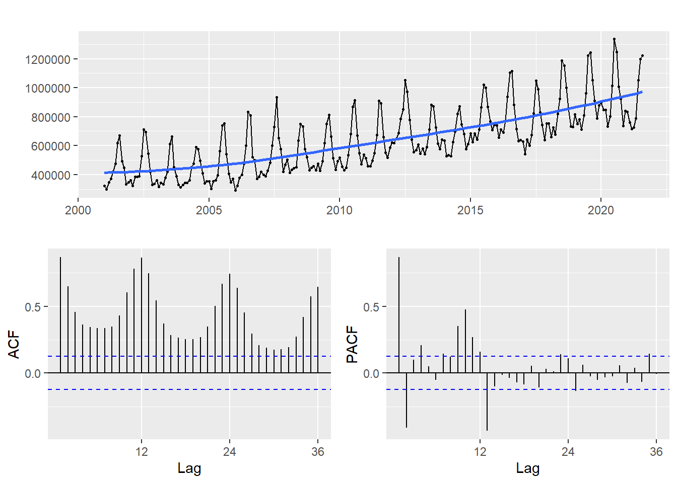

We can clearly see the increasing trend.
There is a visibly strong seasonal variation in our data as well.
It is very obvious that the series is not stationary.
The seasonality is reflected in the ACF plot as well.
Both the ACF and PACF plots show that the lagged values of the series play a very significant role and the series is not stationary.

ggAcf

The ggAcf gives us the Autocorrelation plot. We can similarly, use ggPacf for a Partial Autocorrelation plot.

ggAcf(data, lag.max = 12)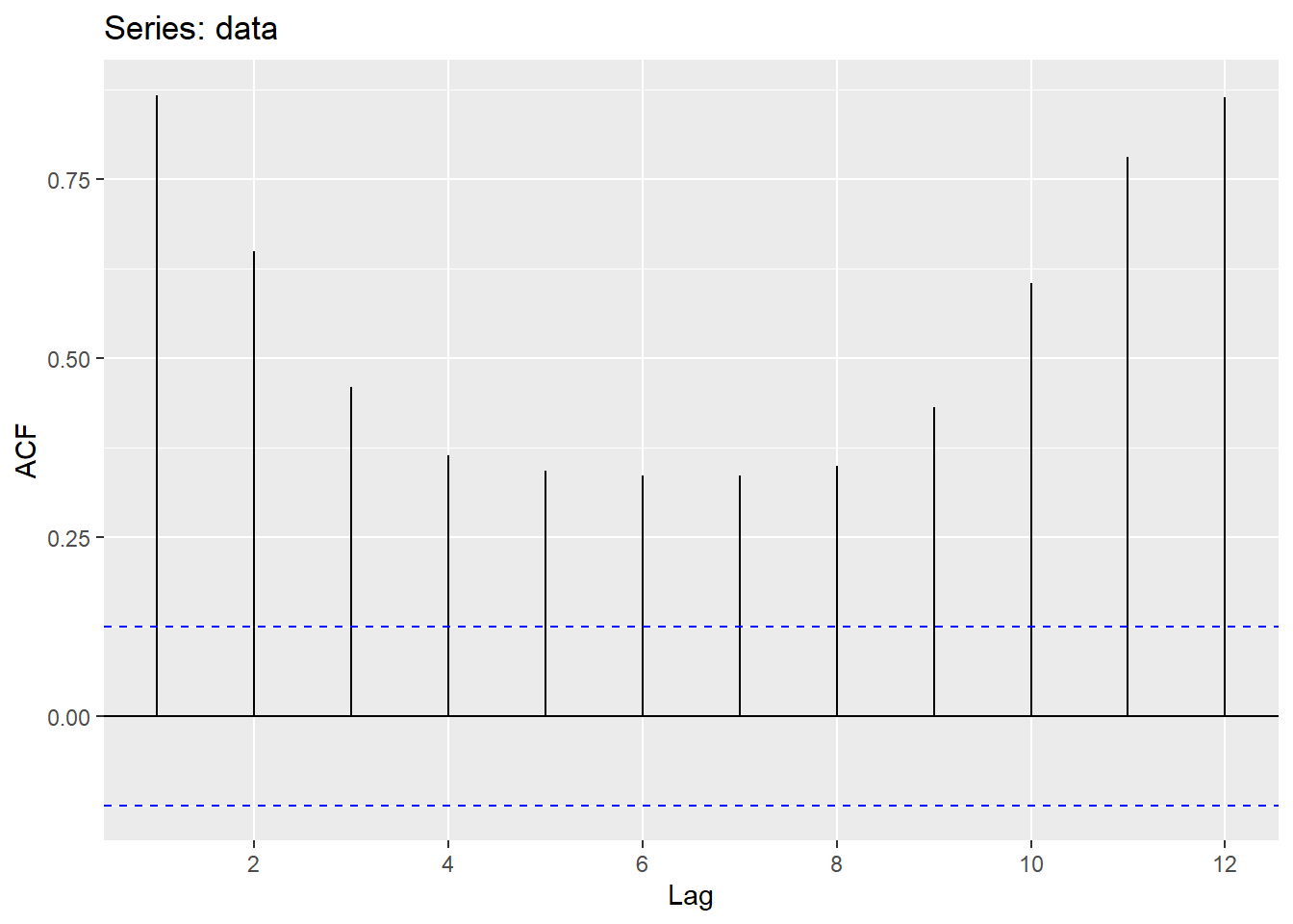

We can specify how many lags we wish to look at using the lag.max argument. Looking at the first 12 lags, we see they are all significant. This is indicative of a strong seasonality. And this makes sense as well because we are dealing with a monthly data set.

ggseasonplot

The ggseasonplot gives us a plot of year-wise seasonal pattern

ggseasonplot(data, year.labels = T)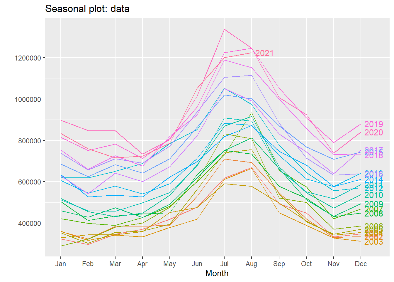

Here, every year gets it’s own curve.
There is a common underlying seasonal pattern, going from left to right, but it is not identical.
There is a bump in consumption in the months of July and August.
While February and November observe visible drop in electricity consumption.
The curve for the year 2021 ends abruptly because our data contains values upto August,2021.

ggsubseriesplot

The ggsubseriesplot gives us a plot also known as Month plot.

ggsubseriesplot(data)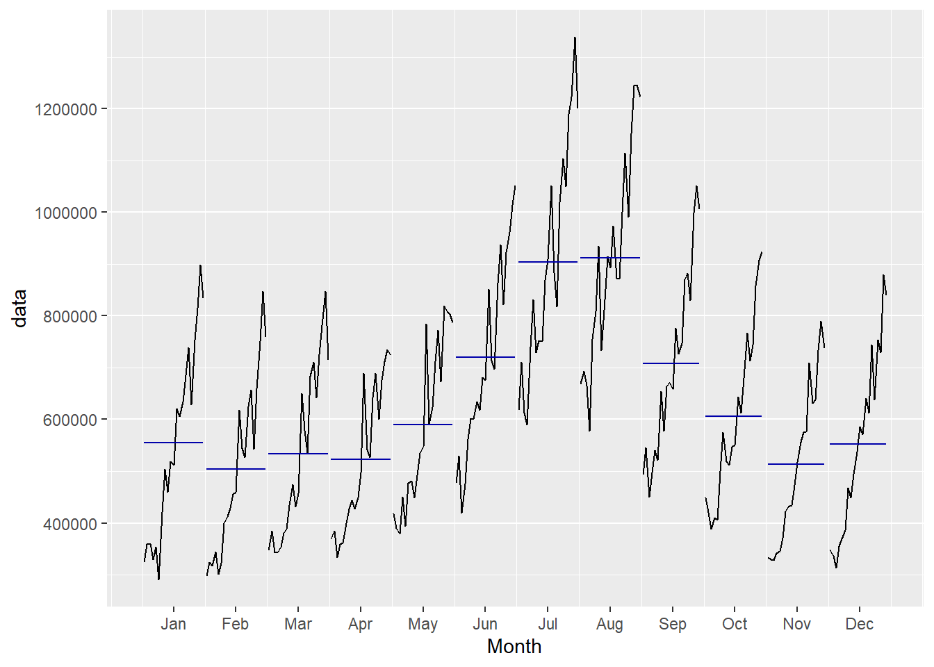

Here, we have a single curve for each month combining data from all years.
For e.g. curve of January has data values of each January from 2001 to 2021.
The horizontal blue line represents the average. So for January, it is the average of all January months over all the years.
We can see the consumption pattern of peaking in the months of July-Aug and falling in Feb-Nov.

gglagplot

The gglagplot gives us plot of \(Y_t\) plotted against different lagged values \(Y_{t-k}\).

gglagplot(data, do.lines = FALSE, lags = 12)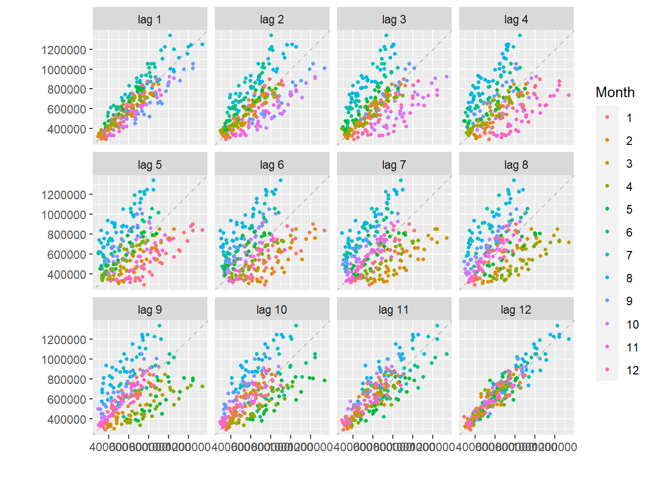

The argument do.lines = FALSE tells R to plot individual data points instead of straight lines.
The closer the values are to the dotted line, the stronger is the relationship.
The strong the relationship, the more important it is to include that lag in our calculations.
Here, all 12 lags show strong positive relationship indicating strong seasonality. This conforms to what we saw above.

STL Decomposition

autoplot(stl(data, s.window = "periodic"))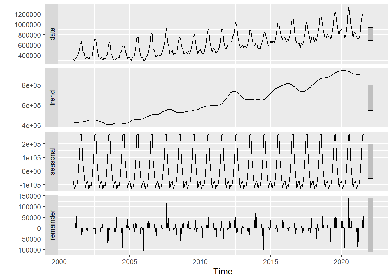

We use STL Decomposition to break down the series into trend, seasonal and random components.
There are thin bars on the right end of every plot. These are called Error Bars. If something lies between the error bars, it is statistically insignificant.
The trend plot shows that there is an overall increase. But the journey is not absolutely linear, there are a few sudden rises and falls.
The seasonal plot tells us that there is significant seasonality in our data and this seasonal pattern repeats itself every year.
The remainder is the what is left after we remove trend and seasonal components from our time series. It should and does seem fairly random.

Let’s fit a SARIMA Model

auto.arima(data) #SARIMA(1,0,1)(0,1,1)[12]

## Series: data 
## ARIMA(1,0,1)(0,1,1)[12] with drift 
## 
## Coefficients:
##          ar1      ma1     sma1     drift
##       0.7982  -0.1586  -0.7700  2230.886
## s.e.  0.0551   0.0925   0.0517   262.937
## 
## sigma^2 estimated as 1.795e+09:  log likelihood=-2852.96
## AIC=5715.91   AICc=5716.18   BIC=5733.23

Equation of fitted SARIMA Model:

\((1-L^S)(1-\phi_ L)Y_t = (1+\theta L)(1+\theta_{S}L^S)e_t\)

Let \(Z_t = (1-L^S)Y_t\)

Then, \(Z_t= \phi_1Z_{t-1} + e_t +\theta_{1S}e_{(t-1)s} +\theta_1 e_{t-1} +\theta_{1S}\theta_1 e_{(t-1)S-1}\)