Neural Networks
Kunal Choudhary
Time isn’t the main thing. It is the only thing - Miles Davis

Introduction
We know how important it is to estimate seasonality of our data, gauge the trend and ensure that the data is stationary. But in practice, the presence of trend and season variation can be hard to estimate and/or remove. It is often very difficult to define trend and seasonality satisfactorily.
The main difficulty is that the underlying dynamics generating the time series is usually unknown and seems random. The traditional statistical time series tools requires considerable experience and skills to select appropriate parameters to capture this underlying dynamics of the data. The great thing about neural networks is that it does not require you to specify the exact nature of relationship (linear or non-linear, seasonality, trend) that exists between input and output.
The Task Of A Neuron is to performed a weighted sum of inputs and apply an activation function before passing the output to the next layer.
Activation Functions
Sigmoid is a ‘s-shaped’ differentiable activation function. It takes a real-valued number and squashes it between 0 and 1 range. It is given by f(u)=1/(1+exp(−cu)).
Sigmoid function can be easily differentiated. This is helps us to reduce the computational cost during training. The derivative is used to learn which weights work best of the network to produce output with minimum mistake.
Hyperbolic Tangent. It is a popular alternative to the sigmoid function. It takes the form f(u)=tanh(cu). It is also ‘s-shaped’ but it produces output between -1, +1 range. Tan h is symmetrical about zero.
Under Modern Deep Learning problems, ReLU is popular function because of its simplicity. It is a piece-wise linear function, it is zero when in the negative regime and it is strictly the identity function in the positive regime.
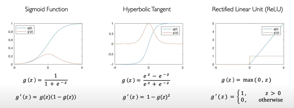
Why do we need Activation Functions?
The purpose of activation functions is to introduce non-linearities into the network.
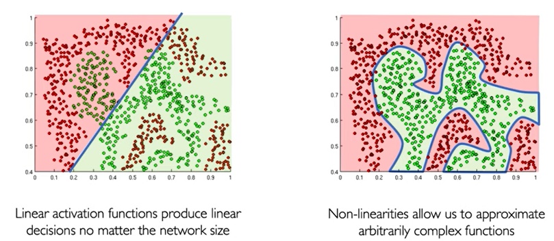
If we use linear activation functions, the separation outcome is poor. But, using non-linear activation functions allows us to approximate arbitrarily complex functions and produce better results.
Feed Forward Neural Network
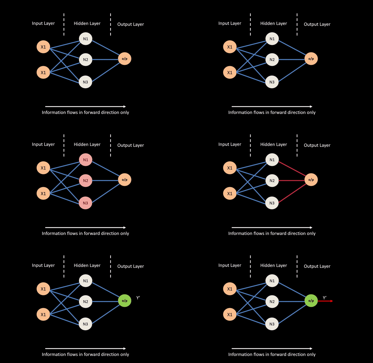
A feed forward neural network is constructed from a number of interconnect nodes called neurons. These are usually arranged into layers. A typical feed-forward network will have at a minimum an input layer, a hidden layer and a output layer.
- Input layers take in attributes / covariates we wish to feed the network.
- Output layer corresponds to the output we wish to predict or classify.
- Hidden layer nodes are generally used to perform non-linear transformation on the original input attributes.
How does a Neural Network Learn?
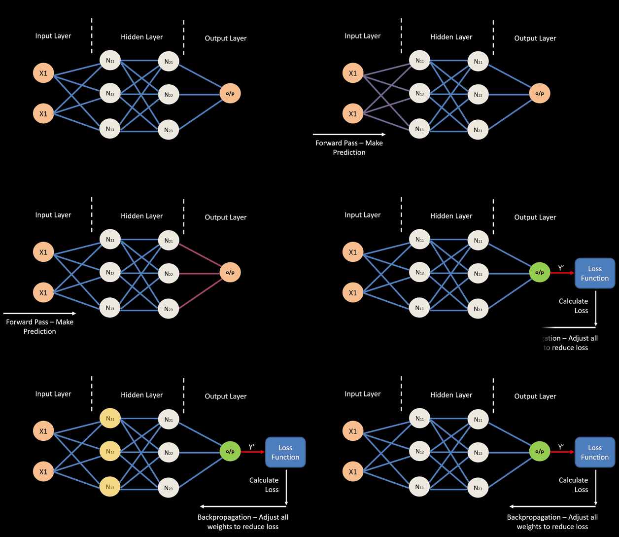
For any input data and neural network weights, there is an associated magnitude of error, which is measured by a cost function. This is the measure of how the neural network performs. The goal is to find a set of weights that minimizes the mismatch between network outputs and actual values.
The typical neural network applies error propagation from output to inputs, gradually fine-tuning i.e. improving the weights by minimizing errors.
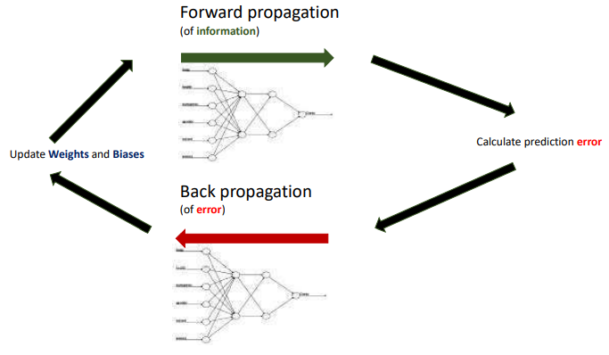
Suppose we have a loss function which contains only 2 weights W0,W1. We can visualize the loss landscape (different values of loss function with respect to W0,W1) as 3D graph as below.
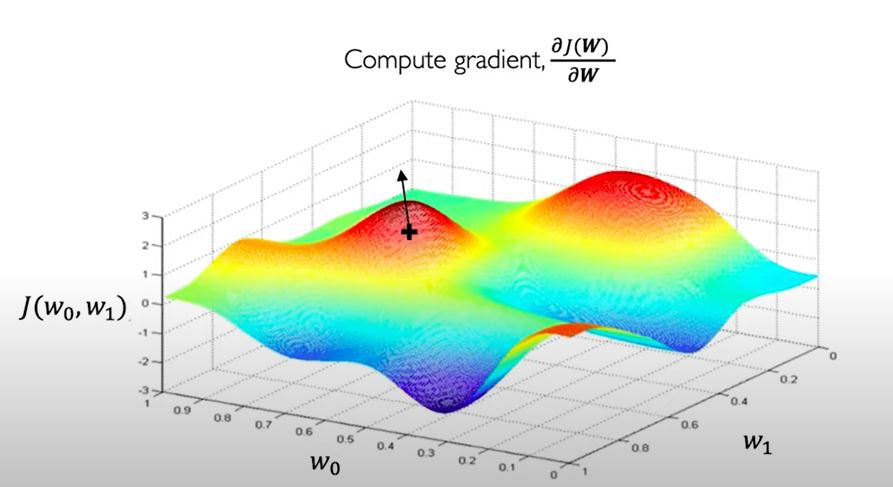
Our aim to find the lowest point in landscape because it corresponds to minimum value of loss function i.e. good performance of the neural network.
We can start at any point, find the derivative of the loss function at that point. This derivative tells us in which direction is upwards, we can take the negative of the derivative to find the downward direction. We take a step in that direction and repeat the process until we converge i.e. reach to the global minimum of the landscape.
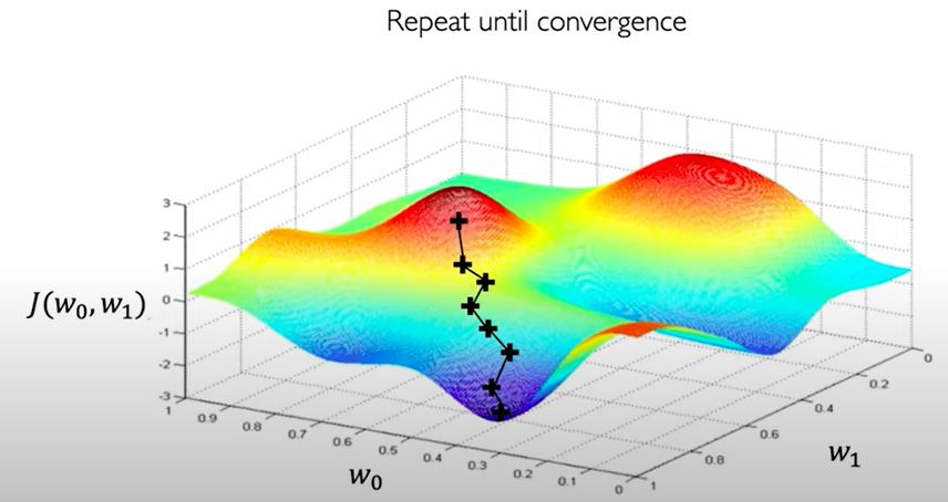
This step is called the Learning Rate which define how big a step we need to take. If we take large steps, then we may miss the global minimum while a small step may trap us in the local minimum preventing us from reaching the global minimum.

Overfitting - A Problem of Generalization
The problem of Generalization in essence means that the network we build should be able to perform well on new unseen data. For this, it should not overfit training data.
To deal with this we can use the idea of Early Stopping where we stop training when we realize the loss is increasing. Increasing of loss is indicative of overfitting.
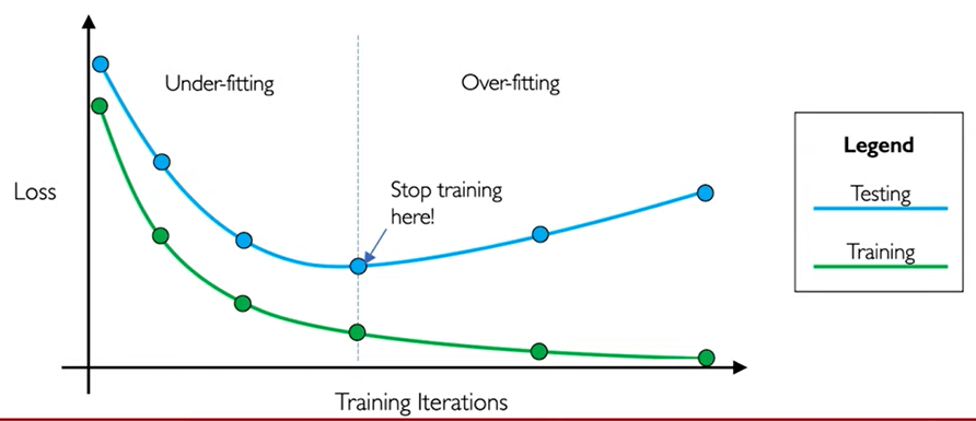
The loss on training set will always go down as long as the network can memorize (i.e. overfit) the training data and simultaneously, the loss on test will increase.
Some Resources for Deeper Understanding
- Youtube : 3Blue1Brown Neural Network
- Youtube : MIT 6S: Introduction to Deep Learning
- Youtube : Dr. Bharatendra Rai
- Book : Neural Networks For Time Series Forecasting With R by N.D Lewis
- Book : Forecasting: Principles and Practice by Rob J Hyndman
- More resource are mentioned throughout the article.